Why use SQL window functions
This is a chapter from my book SQL Window Functions Explained. The book is a clear and visual introduction to the topic with lots of practical exercises.
In short, window functions help you create great analytical reports without Excel or Pandas.
The easiest way to explain this is through concrete examples. We will work with a toy employee table:
┌────┬──────────┬────────┬────────────┬────────┐
│ id │   name   │  city  │ department │ salary │
├────┼──────────┼────────┼────────────┼────────┤
│ 11 │ Diane    │ London │ hr         │ 70     │
│ 12 │ Bob      │ London │ hr         │ 78     │
│ 21 │ Emma     │ London │ it         │ 84     │
│ 22 │ Grace    │ Berlin │ it         │ 90     │
│ 23 │ Henry    │ London │ it         │ 104    │
│ 24 │ Irene    │ Berlin │ it         │ 104    │
│ 25 │ Frank    │ Berlin │ it         │ 120    │
│ 31 │ Cindy    │ Berlin │ sales      │ 96     │
│ 32 │ Dave     │ London │ sales      │ 96     │
│ 33 │ Alice    │ Berlin │ sales      │ 100    │
└────┴──────────┴────────┴────────────┴────────┘
Let's look at some tasks that are convenient to solve using SQL window functions. We'll save the technical details for later chapters. For now, let's review the use cases.
However, if you are eager to start practicing, feel free to skip this chapter and move on to the next one.
Ranking
Ranking means coming up with all kinds of ratings, from the winners of the World Swimming Championships to the Forbes 500.
We will rank employees.
Overall salary rating
Let's rank employees by salary:
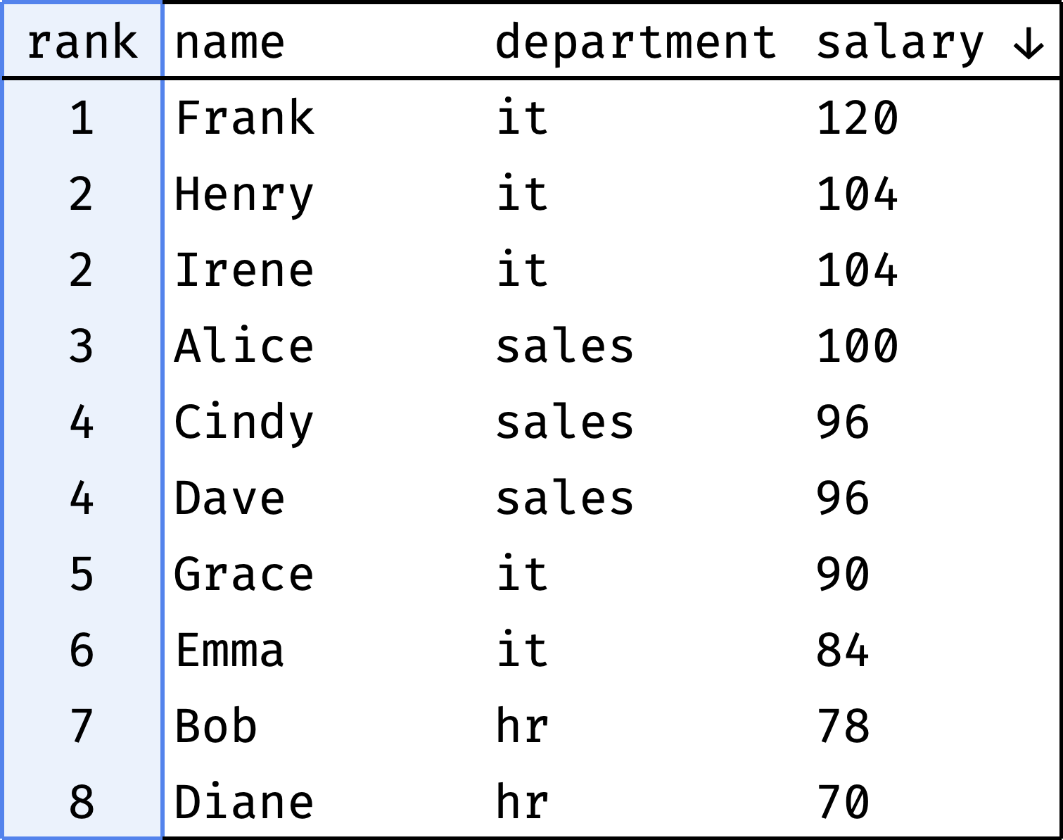
The rank column shows each employee's position in the overall rating.
Some colleagues have the same salary (Henry and Irene, Cindy and Dave) — so they receive the same rank.
Salary rating by department
Similar rating, but created for each department separately instead of the entire company:
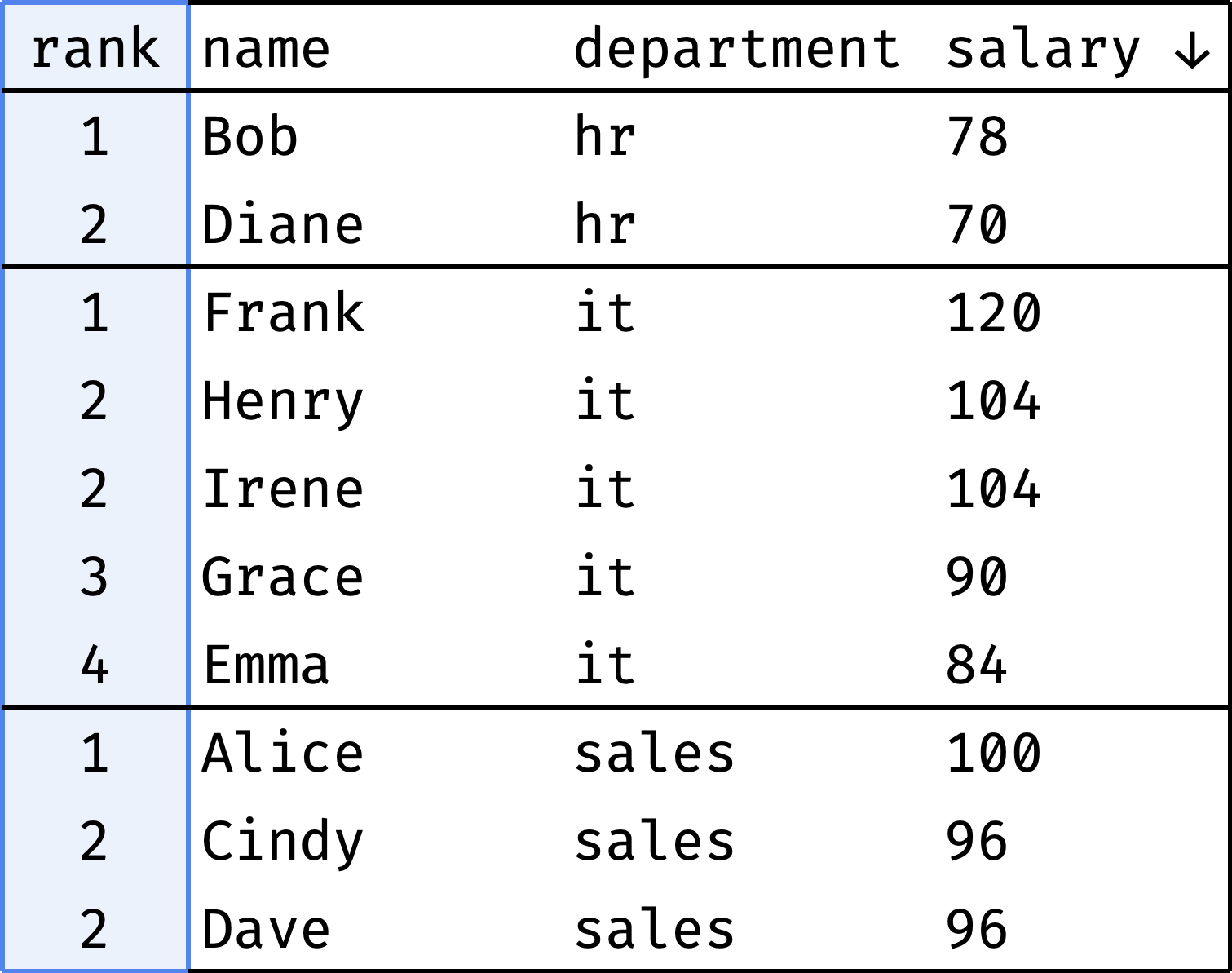
The rank column shows each employee's position in the department's rating.
Salary groups
Let's divide the employees into three groups according to their salary:
- highly-paid,
- medium-paid,
- low-paid.
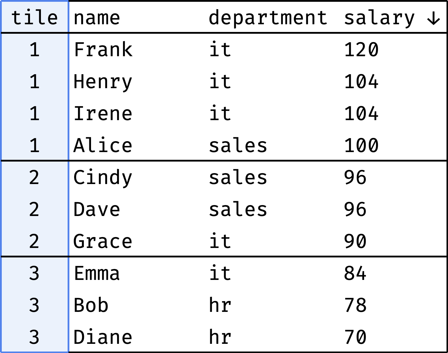
The tile column shows which group each employee belongs to.
The most "precious" colleagues
Let's find the highest-paid people in each department:
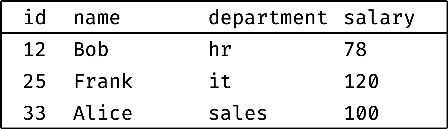
No more salary raises for them, I guess.
Comparing by offset
Comparing by offset means looking at the difference between neighboring values. For example, if you compare the countries ranked 5th and 6th in the world in terms of GDP, how different are they? What about 1st and 6th?
Sometimes we compare with boundaries instead of neighbors. For example, there are 50 top tennis players in the world, and Maria Sakkari is ranked 10th. How do her stats compare to Iga Swiatek, who is ranked 1st? How does she compare to Lin Zhou, who is ranked 50th?
We will compare employees.
Salary difference with the neighbor
Let's arrange employees by salary and see if the gap between neighbors is large:
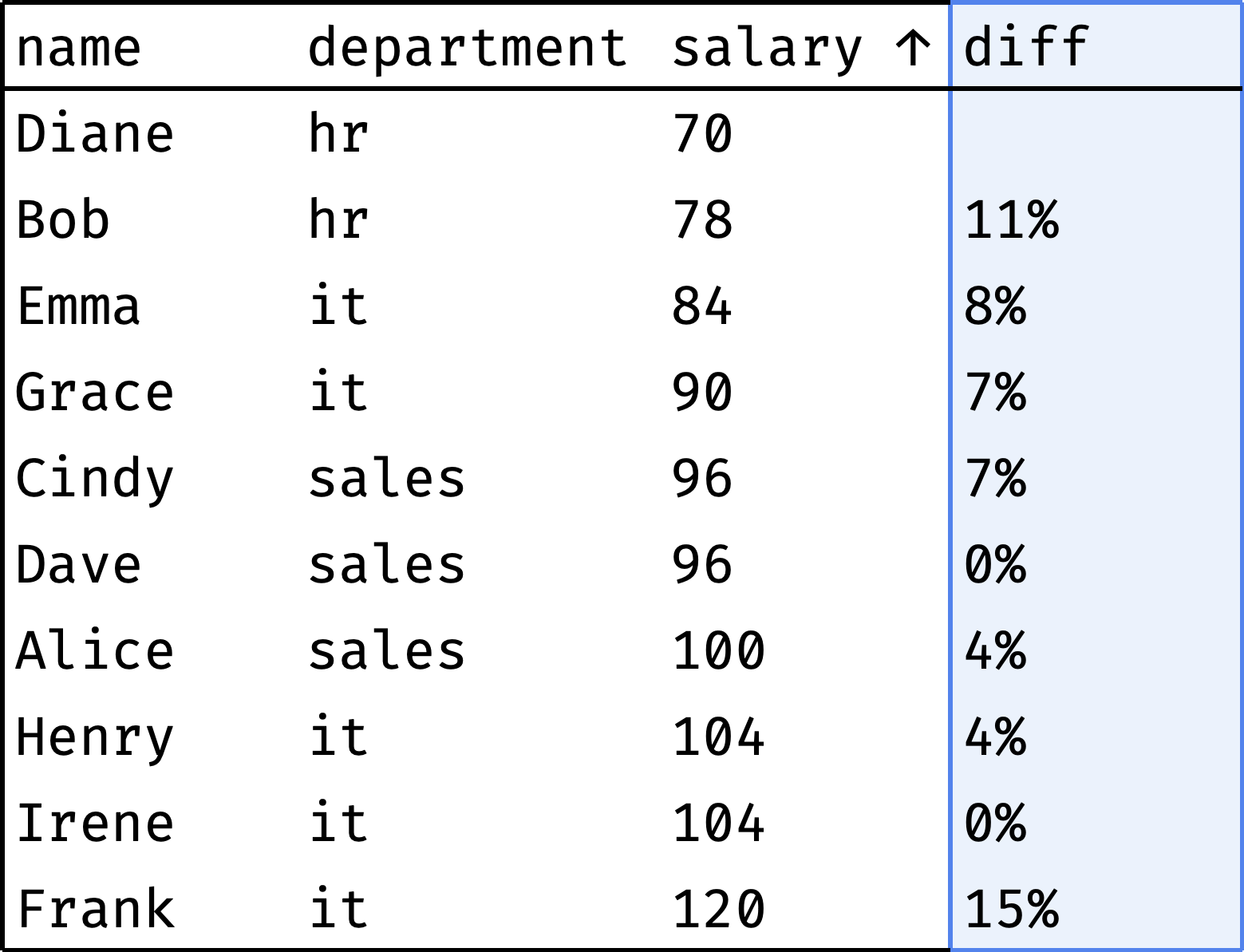
The diff column shows how much the employee's salary differs from the previous colleague's salary. As you can see, there are no significant gaps. The largest ones are Diane and Bob (11%) and Irene and Frank (15%).
Department salary range
Let's see how an employee's salary compares to the minimum and maximum wages in their department:
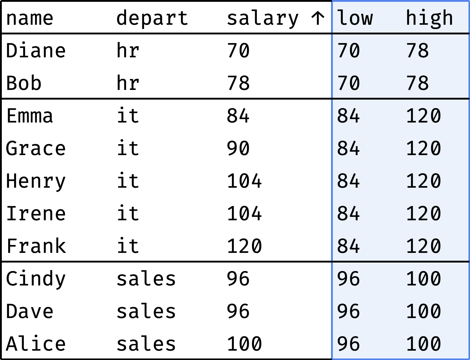
For each employee, the low column shows the minimum salary in the department, and the high column shows the maximum. As you can see, the salary ranges for HR and Sales are narrow, but the range for IT is much wider.
Aggregation
Aggregation means counting totals or averages. For example, the average salary per city. Or the total number of gold medals for each country in the Olympic rankings.
We will aggregate employee salaries.
Comparing with the salary fund
Each department has a salary fund — money spent monthly on paying employees' salaries. Let's see what percentage of this fund represents each employee's salary:
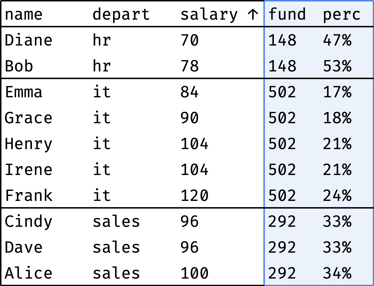
The fund column shows the department's salary fund, and the perc column shows the employee's salary share of that fund. As you can see, everything is more or less even in HR and Sales, but IT has a noticeable spread of salaries.
Comparing to the average salary
I wonder how large is the spread of salaries inside departments. Let's calculate the deviation of each employee's salary from the average department salary:
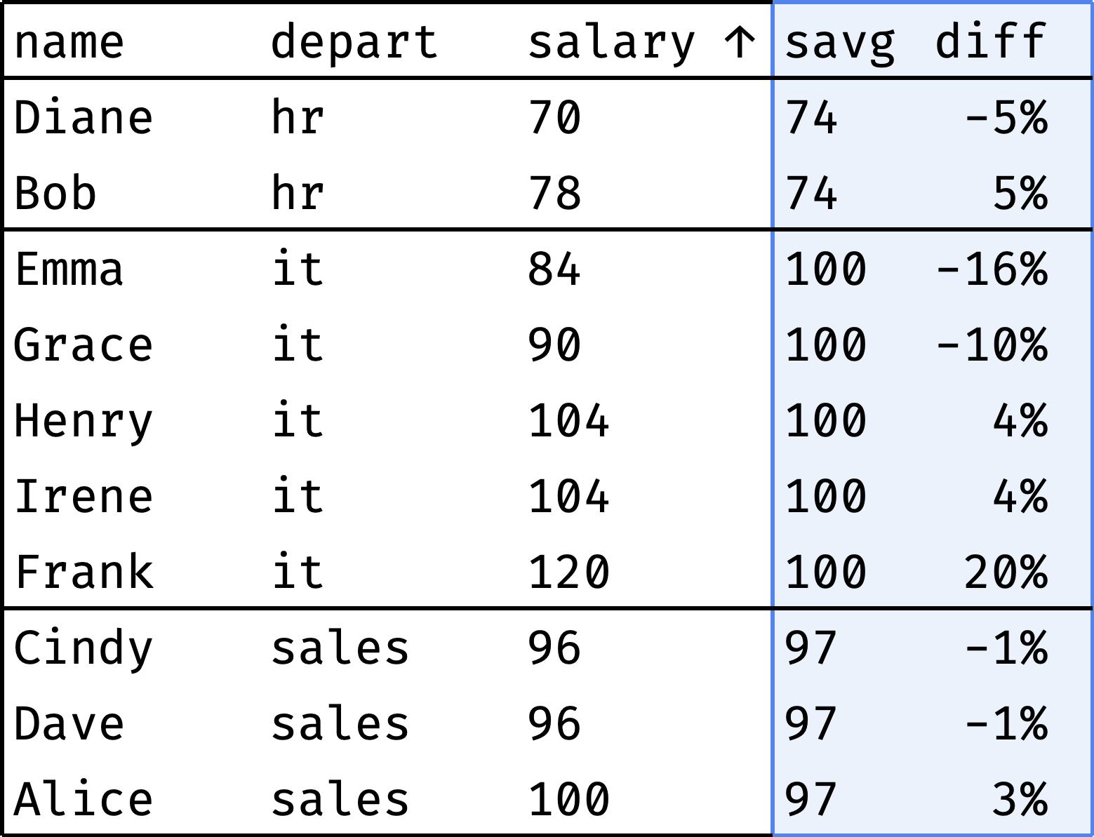
The result confirms the previous observation: IT salaries range from -16% to +20% of the average, while other departments are within 5%.
Rolling aggregates
Rolling aggregates (also known as sliding or moving aggregates) are just totals — sums or averages. But instead of calculating them across all elements, we take a different approach.
Consider the company our employees work for. Here is a table with its income and expenses for nine months of the year:
┌──────┬───────┬────────┬─────────┐
│ year │ month │ income │ expense │
├──────┼───────┼────────┼─────────┤
│ 2020 │ 1     │ 94     │ 82      │
│ 2020 │ 2     │ 94     │ 75      │
│ 2020 │ 3     │ 94     │ 104     │
│ 2020 │ 4     │ 100    │ 94      │
│ 2020 │ 5     │ 100    │ 99      │
│ 2020 │ 6     │ 100    │ 105     │
│ 2020 │ 7     │ 100    │ 95      │
│ 2020 │ 8     │ 100    │ 110     │
│ 2020 │ 9     │ 104    │ 104     │
└──────┴───────┴────────┴─────────┘
Expenses moving average
Judging by the data, the income is growing: 94 in January → 104 in September. But are the expenses growing as well? It's hard to tell right away: expenses vary from month to month. To smooth out these spikes, we'll use the "3-month average" — the average between the previous, current, and next month's expenses for each month:
- moving average for February = (January + February + March) / 3;
- for March = (February + March + April) / 3;
- for April = (March + April + May) / 3;
- etc.
Let's calculate the moving average for all months:
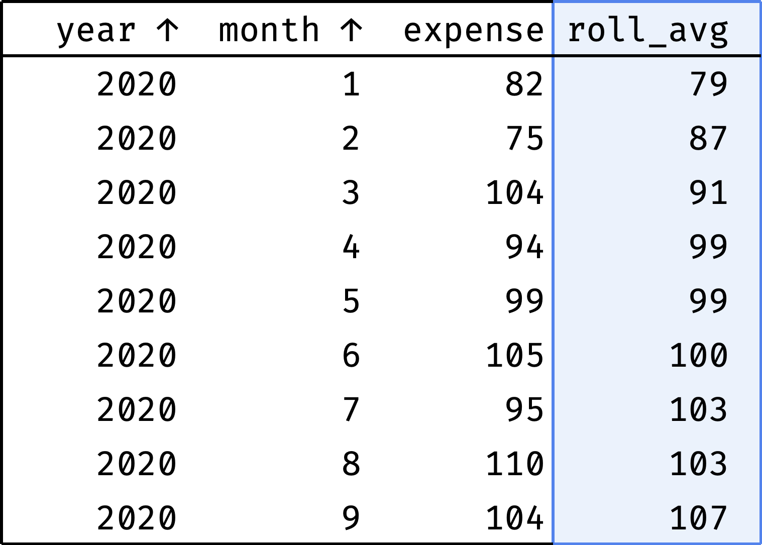
Now it is clear that expenses are steadily growing.
Cumulative income
Thanks to the moving average, we know that income and expenses are growing. But how do they relate to each other? We want to understand whether the company is "in the black" or "in the red", considering all the money earned and spent.
It is essential to see the values for each month, not only for the end of the year. If everything is OK at the end of the year, but the company went negative in June — this is a potential problem (companies call this situation a "cash gap").
Let's calculate income and expenses by month as a cumulative total:
- cumulative income for January = January;
- for February = January + February;
- for March = January + February + March;
- for April = January + February + March + April;
- etc.
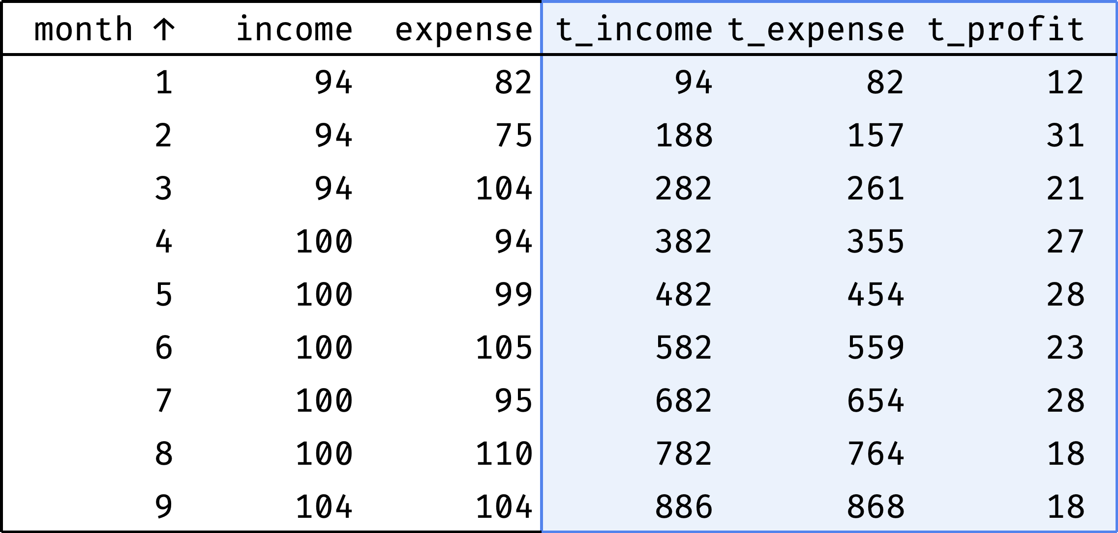
Now it is clear that the company is doing well. In some months, expenses exceed income, but there is no gap due to the accumulated cash reserve.
Summary
SQL window functions help to solve the following tasks:
- Ranking (all kinds of ratings).
- Comparing by offset (neighboring elements and boundaries).
- Aggregation (sum and average).
- Rolling aggregates (sum and average in dynamics).
Of course, this is not an exhaustive list. But I hope it is now clear why window functions are useful for data analysis. In the next chapter, we will examine what windows are and how to use them.
★ Subscribe to keep up with new posts.